How to Analyze a CSV File with Python and Pandas

CSV files show up in almost every business workflow. You may export orders from an ecommerce platform, download leads from a CRM, receive finance data from another team, or pull product usage data from an internal dashboard.

The challenge is that a raw CSV file rarely answers a question directly. It may contain duplicate rows, missing values, inconsistent column names, and dates stored in a format that makes time analysis difficult.

In this tutorial, you will work through a realistic sales analysis project. Imagine you received an ecommerce order export and need to answer one practical question:

What can this CSV tell us about revenue by product, category, country, and month?

You will start with a raw CSV file and finish with cleaned data, useful summaries, visualizations, and exported result files.

By the end, you will have:

• Loaded a CSV file into Pandas
• Inspected rows, columns, data types, and missing values
• Cleaned column names, duplicates, missing values, and data types
• Created a revenue column
• Used filtering, sorting, and groupby() to answer business questions
• Created a category bar chart and monthly line chart
• Exported cleaned data and summary CSV files

Prerequisites

You should know basic Python syntax, including variables, function calls, imports, and running scripts or notebook and you do not need previous Pandas experience.

You can follow along in Jupyter Notebook, Google Colab, VS Code, or a regular Python script. A notebook gives you the easiest learning experience because you can inspect each result as you go.

Install Pandas and Matplotlib:

python -m pip install pandas matplotlib

If you use Conda, install from conda-forge:

conda install -c conda-forge pandas matplotlib

Now import the libraries:

import pandas as pd
import matplotlib.pyplot as plt

Check your Pandas version:

print(pd.__version__)

You may see output like this:

3.0.3

This tutorial uses modern Pandas practices. You will avoid chained assignment, and you will not use inplace=True as the default way to update data. Direct assignment usually reads better and works well with current Pandas behavior.

If Python raises ModuleNotFoundError: No module named ‘pandas’, your editor and terminal may use different Python environments. In VS Code, check the selected interpreter. In Jupyter, check the active kernel.

Create the Sales CSV File

You will use one dataset throughout this tutorial: a small ecommerce sales export. Keeping the dataset small lets you see every row, but the workflow matches what you would do with a larger real-world CSV. Either use a sale csv file you have, create a sample one or use this example to follow along

The dataset includes the columns you would expect in a sales export: order ID, order date, product, category, quantity, unit price, customer country, and payment method. It also includes a few issues on purpose. One row appears twice, one order has no date, one order has no category, and one order has no unit price.

Those issues are useful. They let you practice the kind of judgment you need when analyzing real CSV files. 

Load the CSV File With Pandas

Load the file with pd.read_csv():

df = pd.read_csv(
    "sales_data.csv",
    parse_dates=["Order Date"]
)

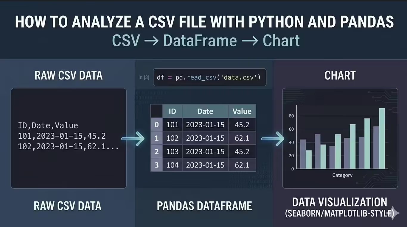
print(df.head())

Expected output:

This code creates a DataFrame named df. A DataFrame is Pandas’ table structure: rows represent records, and columns represent fields.

The parse_dates=[“Order Date”] argument matters because you will analyze monthly revenue later. If you load dates as plain text, you create extra work for yourself.

Understand File Paths

The path “sales_data.csv” is a relative path. It means Python should look for the file in the folder where your code runs.

If your file lives somewhere else, use an absolute path. On Windows, that might look like this:

df = pd.read_csv(
    r"C:\Users\YourName\Downloads\sales_data.csv",
    parse_dates=["Order Date"]
)

For this project, I would encourage you to use relative paths. They make your analysis easier to move between folders, machines, and teammates.

Useful read_csv() Options

You do not need many options for this sample file, but real CSV files often need extra instructions.

df = pd.read_csv(
    "sales_data.csv",
    sep=",",
    encoding="utf-8",
    parse_dates=["Order Date"],
    na_values=["", "NA", "N/A", "null"]
)

Here is the practical rule:

Use sep when the delimiter is not a comma, use encoding when the file fails to decode, use na_values when the source system uses custom labels for missing values. parse_dates to make a column behave like a date.

You will see usecols, dtype, and chunksize later when you adapt the workflow to larger files.

If you get FileNotFoundError, Pandas cannot find the file from the current working folder. Run print(Path.cwd()), move the CSV there, or use a full path.

If the file loads as one giant column, try a different delimiter such as sep=”;” or sep=”\t”.

If Pandas raises UnicodeDecodeError, try encoding=”latin1″ or ask the data owner for the file encoding.

Inspect the Data Before You Clean It

Before you clean anything, inspect the dataset. This step protects you from making lazy assumptions.

Start with the first rows:

print(df.head())

Then check the last rows:

print(df.tail())

head() confirms that the file loaded as expected. tail() helps you catch issues near the bottom of the file. In this dataset, the last row repeats order 1008, which hints at a duplicate.

Expected result for tail

Check the size:

print(df.shape)

Expected output:

(16, 8)

The raw dataset has 16 rows and 8 columns.

Inspect the column names:

print(df.columns)

Expected output:

The names make sense to a human, but they are awkward in code because they contain spaces and mixed capitalization.

Now use info():

df.info()

Expected output will look similar to this:

This tells you where the main data quality issues are. You have missing values in Order Date, Category, and Unit Price.

Use describe() to inspect numeric columns:

print(df.describe())

Look for values that violate common business rules: negative quantities, zero prices, or extreme outliers. In this small file, the numeric ranges look reasonable.

Finally, check exact data types:

print(df.dtypes)

Your text-column dtypes may vary slightly by Pandas version. 

Focus on the important question: can Pandas treat dates as dates and numbers as numbers?

If Order Date appears as object or str, Pandas did not parse it as a date. Check that parse_dates=[“Order Date”] matches the column name exactly.

Clean the CSV Data

Now clean the file so you can trust the analysis. Cleaning does not mean forcing the data to look perfect. It means making clear, documented decisions that support your questions. We will start with the column.

Clean Column Names

Clean names early because every later step uses these names.

df.columns = (
    df.columns
    .str.strip()
    .str.lower()
    .str.replace(" ", "_")
)

print(df.columns)

Expected output:

Now your code can use df[“unit_price”] instead of df[“Unit Price”].

This may look cosmetic, but it is practical. Clean column names reduce typing errors and make your code easier to scan.

Count Missing Values

Count missing values after cleaning the column names:

print(df.isna().sum())

Expected output:

This output gives you three separate cleaning decisions. A missing date, missing category, and missing price do not mean the same thing. Treating them the same way would create weak analysis.

Remove Duplicate Rows

Check exact duplicates:

print(df.duplicated().sum())

Expected output:

1

Remove the duplicate row:

df = df.drop_duplicates()
print(df.shape)

Expected output:

(15, 8)

You now have 15 rows.

This is safe here because the duplicate row matches exactly. In a real dataset, duplicate IDs with different values require investigation, so do not delete those blindly.

Handle Missing Dates

We want monthly revenue, so rows without dates cannot support one of the main goals. Drop rows where order_date is missing:

df = df.dropna(subset=["order_date"])
print(df["order_date"].isna().sum())

Expected output:

0

This choice is specific to our sale file. If your analysis did not use dates, you might keep the row.

Fill Missing Categories

A missing category should not erase a valid sale. Keep the row and label the missing value as unknown:

df["category"] = df["category"].fillna("Unknown")
print(df["category"].value_counts(dropna=False))

Expected output should show one Unknown category.

This lets you include the revenue while still exposing the data-quality issue. That is usually better than hiding the row or pretending you know the category.

Fill Missing Unit Prices

A missing price affects revenue, so you need a reasonable rule. For this dataset, fill the missing price with the median price of the same product:

df["unit_price"] = df["unit_price"].fillna(
    df.groupby("product")["unit_price"].transform("median")
)

print(df["unit_price"].isna().sum())

Expected output:

0

The important method here is transform(“median”). It calculates a median unit price for each product and returns values aligned to the original rows. That alignment lets Pandas fill the missing price with the right product-level median.

This beats a global median because product prices are not interchangeable. A monitor price and a cable price should not influence a missing notebook price.

Confirm and Fix Data Types

Check data types again:

print(df.dtypes)

Convert text columns to Pandas string type:

df = df.astype({
    "product": "string",
    "category": "string",
    "customer_country": "string",
    "payment_method": "string"
})

For this sample file, quantity and unit_price should already be numeric. For real files, convert numeric columns explicitly when needed:

df["quantity"] = pd.to_numeric(df["quantity"], errors="coerce")
df["unit_price"] = pd.to_numeric(df["unit_price"], errors="coerce")

Then check whether conversion introduced missing values:

print(df[["quantity", "unit_price"]].isna().sum())

Use errors=”coerce” when you want invalid numeric text to become missing values. That makes the problem visible.

Create a Revenue Column

Create the metric you will use for analysis:

df["total_sales"] = df["quantity"] * df["unit_price"]
print(df[["order_id", "quantity", "unit_price", "total_sales"]].head())

Expected output:

At this point, the dataset has moved from raw order records to analysis-ready sales data.

Cleaning Checkpoint

Before analysis, run one quick checkpoint:

print(df.shape)
print(df.isna().sum())
print(df.dtypes)

You should see 14 rows after removing one duplicate and one row without a date. You should also see no missing values in the fields needed for this project.

This checkpoint separates cleaning from analysis. You do not want to discover data-quality problems halfway through a revenue summary.

Analyze Sales With groupby()

From now you can start answering business questions. The main tool in this section is groupby(). In plain English, groupby() lets you split rows into groups, calculate something for each group, and combine the results into a summary table.

For example, when you group by category and sum revenue, Pandas does this:

1. Splits rows into category groups.
2. Adds total_sales inside each category.
3. Returns one row per category.

Calculate Total Revenue

Start with the headline metric:

total_revenue = df["total_sales"].sum()
print(f"Total revenue: ${total_revenue:,.2f}")

Expected output:

Total revenue: $1,333.57

This is the total revenue after cleaning. It excludes the duplicate row and the row without an order date.

Find Revenue by Category

Group by category:

category_sales = (
    df.groupby("category", as_index=False)["total_sales"]
    .sum()
    .sort_values("total_sales", ascending=False)
)

print(category_sales)

Expected output:

as_index=False keeps category as a normal column instead of turning it into the index. For beginner analysis and CSV exports, that format is easier to read and reuse. Furniture leads revenue, even though it has fewer orders than some other categories. High unit prices can matter more than order count.

Find Top Products

Now summarize by product:

product_sales = (
    df.groupby("product", as_index=False)
    .agg(
        total_sales=("total_sales", "sum"),
        units_sold=("quantity", "sum"),
        orders=("order_id", "count")
    )
    .sort_values("total_sales", ascending=False)
)

print(product_sales)

Expected output:

This table is more useful than a single revenue ranking. It shows revenue, units sold, and order count together. The Monitor generated the most revenue. USB-C Cable sold the most units. Those are different types of performance, and a good analyst keeps them separate.

Find Revenue by Country

Group by customer country:

country_sales = (
    df.groupby("customer_country", as_index=False)["total_sales"]
    .sum()
    .sort_values("total_sales", ascending=False)
)

print(country_sales)

Expected output:

The United States contributes the most revenue in this sample. In a real business, this kind of table can support regional reporting, marketing decisions, or logistics planning.

Analyze Monthly Revenue

Create a month column from order_date:

df["order_month"] = df["order_date"].dt.to_period("M").astype("string")

The .dt accessor lets you work with datetime values. to_period(“M”) converts each date to its month, such as 2026-03. That gives you a clean monthly grouping key.

Now summarize revenue by month:

monthly_sales = (
    df.groupby("order_month", as_index=False)["total_sales"]
    .sum()
    .sort_values("order_month")
)

print(monthly_sales)

Expected output:

Revenue rises in March and April because the dataset includes higher-priced furniture orders in those months.

If .dt raises an error, order_date is not a datetime column. Convert it with:

df["order_date"] = pd.to_datetime(df["order_date"], errors="coerce")

Then check df[“order_date”].isna().sum() before continuing.

Filter High-Value Orders

Use filtering to inspect the rows behind your summary tables.

high_value_orders = df[df["total_sales"] >= 100].sort_values(
    "total_sales",
    ascending=False
)

print(high_value_orders[["order_id", "product", "customer_country", "total_sales"]])

Expected output:

Only a few orders drive a large share of revenue. This is the kind of detail that summary tables can hide.

For multiple conditions, wrap each condition in parentheses:

us_high_value_orders = df[
    (df["customer_country"] == "United States") &
    (df["total_sales"] >= 100)
]

print(us_high_value_orders[["order_id", "product", "total_sales"]])

Use & for “and” and | for “or”. Python’s and and or do not work for Pandas Series filters.

Visualize the Results

You should not chart everything. Chart the results that become easier to understand visually.

Category Revenue Bar Chart

Use a bar chart for category comparison:

category_sales.plot(
    kind="bar",
    x="category",
    y="total_sales",
    legend=False,
    title="Revenue by Category"
)

plt.xlabel("Category")
plt.ylabel("Revenue")
plt.tight_layout()
plt.show()

The chart should show Furniture as the highest-revenue category. A stakeholder could understand that pattern faster from the chart than from the table.

Monthly Revenue Line Chart

Use a line chart for time trends:

monthly_sales.plot(
    kind="line",
    x="order_month",
    y="total_sales",
    marker="o",
    legend=False,
    title="Monthly Revenue"
)

plt.xlabel("Month")
plt.ylabel("Revenue")
plt.tight_layout()
plt.show()

The line should rise in March and April. In a larger dataset, this chart would help you identify seasonality, campaign effects, or unexpected drops.

If charts do not appear, make sure Matplotlib is installed and call plt.show(). In Jupyter notebooks, %matplotlib inline can help, but do not use that line in a regular Python script.

Working With Larger CSV Files

This tutorial uses a small file so you can focus on the workflow. Real CSV files may contain hundreds of thousands or millions of rows. You can still use Pandas, but you should load the data more carefully.

If you only need some columns, use usecols:

columns_to_load = [
    "Order ID",
    "Order Date",
    "Product",
    "Category",
    "Quantity",
    "Unit Price",
    "Customer Country"
]

large_df = pd.read_csv(
    "sales_data.csv",
    usecols=columns_to_load,
    parse_dates=["Order Date"]
)

This reduces memory use and keeps your analysis focused.

If you know the schema, set data types while loading:

large_df = pd.read_csv(
    "sales_data.csv",
    usecols=columns_to_load,
    parse_dates=["Order Date"],
    dtype={
        "Product": "string",
        "Category": "string",
        "Customer Country": "string",
        "Quantity": "int64",
        "Unit Price": "float64"
    }
)

If you are unsure about types, load a small sample first:

sample_df = pd.read_csv("sales_data.csv", nrows=1000)
print(sample_df.dtypes)
For very large files, read in chunks:

revenue_by_country = {}

for chunk in pd.read_csv(
    "sales_data.csv",
    parse_dates=["Order Date"],
    chunksize=5
):

    chunk.columns = (
        chunk.columns
        .str.strip()
        .str.lower()
        .str.replace(" ", "_")
    )

    chunk = chunk.dropna(subset=["order_date", "unit_price"])
    chunk["total_sales"] = chunk["quantity"] * chunk["unit_price"]
    chunk_summary = chunk.groupby("customer_country")["total_sales"].sum()

    for country, revenue in chunk_summary.items():

        revenue_by_country[country] = revenue_by_country.get(country, 0) + revenue

print(revenue_by_country)

The example uses chunksize=5 only because the sample file is tiny. For real files, try chunksize=50_000 or 100_000.

Pandas also supports dtype_backend=”pyarrow”:

df_arrow = pd.read_csv(
    "sales_data.csv",
    dtype_backend="pyarrow"
)

Treat this as optional. It can help some larger workflows, but it may require PyArrow and does not need to be your first optimization.

Pandas is enough for many CSV analysis tasks. If your data outgrows memory or you need fast SQL over local files, look at DuckDB, If you want a fast DataFrame library, consider Polars. Use Dask if you need larger-than-memory workflows with familiar Pandas-like pattern. If many people need shared reporting, use a database.

Export Your Cleaned Data and Summaries

Now finish the project by saving your work.

Save the cleaned dataset:

df.to_csv("cleaned_sales_data.csv", index=False)

Save the summary tables:

category_sales.to_csv("category_sales.csv", index=False)product_sales.to_csv("product_sales.csv", index=False)country_sales.to_csv("country_sales.csv", index=False)monthly_sales.to_csv("monthly_sales.csv", index=False)

Use index=False because the DataFrame index does not contain business information. If you omit it, Pandas writes the index to the file. When you load that file later, you may see an unwanted Unnamed: 0 column.

Confirm that your output files exist:

output_files = [
    "cleaned_sales_data.csv",
    "category_sales.csv",
    "product_sales.csv",
    "country_sales.csv",
    "monthly_sales.csv"
]

for file_name in output_files:

    print(file_name, Path(file_name).exists())

Expected output:

You now have files you can share, inspect in a spreadsheet, or use in another analysis step.

If Pandas raises a permission error, close the file in Excel or any other program that may have locked it.

Common Mistakes When Analyzing CSV Files

Most beginner CSV problems come from file setup, data types, and cleaning decisions.

If Pandas cannot find your file, check your working folder:

print(Path.cwd())

If the CSV loads as one giant column, specify the delimiter:

df = pd.read_csv("sales_data.csv", sep=";")

Use thisiIf the file fails with a decoding error, try another encoding:

df = pd.read_csv("sales_data.csv", encoding="latin1")

If dates do not work with .dt, parse them:

df["order_date"] = pd.to_datetime(df["order_date"], errors="coerce")

Convert numeric columns to load as text with:

df["unit_price"] = pd.to_numeric(df["unit_price"], errors="coerce")

If you need to update values conditionally, use .loc:

df.loc[df["category"].isna(), "category"] = "Unknown"

Avoid this chained-assignment pattern:

df["category"][df["category"].isna()] = "Unknown"

If your exported CSV contains an Unnamed: 0 column, export with:

df.to_csv("cleaned_sales_data.csv", index=False)

A good habit solves many of these mistakes, inspect before cleaning, and recheck after cleaning.

Best Practices Checklist

Here is a best practice checklist I have compiled and encourage you to use this checklist when you analyze your own CSV files:

• Keep the raw file unchanged.
• Inspect the dataset before cleaning it.
• Clean column names early.
• Parse dates before time-based analysis.
• Treat missing values based on column meaning.
• Check duplicates before removing them.
• Convert data types deliberately.
• Create calculated columns for the metrics you need.
• Write analysis around specific questions.
• Sort summary tables before interpreting them.
• Use charts only when they clarify a pattern.
• Save cleaned data separately.
• Export with index=False unless the index matters.

Practice Exercise

Extend the analysis with three questions. First, find revenue by payment method:

payment_sales = (
    df.groupby("payment_method", as_index=False)["total_sales"]
    .sum()
    .sort_values("total_sales", ascending=False)
)

print(payment_sales)

Next, find which country bought the most units:

country_units = (
    df.groupby("customer_country", as_index=False)["quantity"]
    .sum()
    .sort_values("quantity", ascending=False)
)

print(country_units)

Finally, calculate the share of revenue from Furniture:

furniture_revenue = df.loc[
    df["category"] == "Furniture",
    "total_sales"
].sum()

furniture_share = furniture_revenue / df["total_sales"].sum()

print(f"Furniture revenue share: {furniture_share:.1%}")

Export the payment summary:

payment_sales.to_csv("payment_sales.csv", index=False)

This exercise follows the same pattern as the main project: ask a question, group or filter the data, calculate the metric, sort the result, and save the output.

What Learned Today

You started with a raw ecommerce CSV and turned it into a practical sales analysis. You created sales_data.csv, loaded it into Pandas, inspected its structure, cleaned column names, removed a duplicate row, handled missing dates, categories, and prices, and created a total_sales metric.

Then you used that cleaned data to answer business questions about total revenue, category performance, product performance, country revenue, monthly trends, and high-value orders. You also created two charts and exported cleaned and summarized CSV files.

The final files are:

• cleaned_sales_data.csv
• category_sales.csv
• product_sales.csv
• country_sales.csv
• monthly_sales.csv

Conclusion

You analyzed a CSV file with Python and Pandas by following a repeatable workflow: load, inspect, clean, calculate, analyze, visualize, and export. Use the same structure with your own CSV files. Replace the sample file, update the column names, define your questions, and adapt the cleaning rules to your data. The specific dataset will change, but the habit stays the same: understand the file before you trust the numbers.